Classifications with a Support Vector Machine
We offer private, customized training for 3 or more people at your site or online.
In part 1 of this tutorial, we installed the Anaconda distribution of Python and configured it using Conda. We then executed a new notebook with Jupyter Notebooks.
In part 2 of this series, we will configure a Support Vector Machine to perform classifications using data from the Scikit-learn digits sample dataset.
What is a Support Vector Machine?
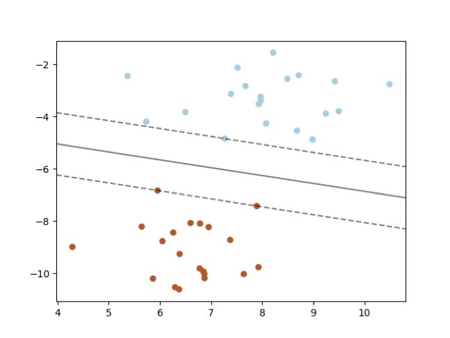
A Support Vector Machine (SVM) is used for either regression or classification models. When performing classification, an SVM is used to create a Support Vector Classifier (SVC) to determine a hyperplane. This divides a set of data into various classifications. Data on one side the hyperplane is one class, and the data on the other side of the hyperplane is another class. A hyperplane is a shape that is one dimension less than the number of data features being used to perform the classification.

Source: http://scikit-learn.org/stable/_images/sphx_glr_plot_separating_hyperplane_0011.png
For example, in the above graphic, the data has two dimensions (features): X1 (on the x-axis) and X2 (on the y-axis). The hyperplane is a line that is one-dimensional (a line is one dimension less than the two dimensions of the data). In the diagram above, the line (hyperplane) is the solid black line. The color of the dots represents the targeted outcomes (classifications). All the light blue dots are on top and the brown dots are on bottom. The line between the two colors of dots indicates that all dots above the line will be classified as light blue and all dots below the line will be classified as brown.
Above and below the solid black line are dashed lines. The distance between the dashed line and the solid black line represents the margin. When the black line is calculated, the SVM seeks to maximize the margin on both sides of the line relative to the vectors closest to it. The vectors close to it are known as the support vectors, as they determine the location of the line.
To calculate the decision surface (it can be a straight or curvy boundary), a kernel function is selected, and each kernel function uses hyperparameters (hyperparameters vs. parameters are explained a little later) and the data features to determine the line. The term decision surface is used because SVM supports a high dimensionality of features meaning the shape is rarely a line; rather, it is some type of multi-dimensional surface.
With a good understanding of a Support Vector Machine and Classifier, let's proceed with the tutorial.
Step 1. Training a Model and Predicting Numbers
Step 1.1 To get started, create a new Python notebook named "Predict a Number".
Step 1.2 In the first notebook cell, type the following line of code:
?from sklearn import datasets, svm
The sklearn module is part of the scikit-learn package installed in the first tutorial using Conda.
The sklearn module provides access to the datasets and various machine learning APIs. There are several "toy" datasets from which to choose, including the images of digits, data from iris flowers, and Boston-area housing prices data.
For More Information on All Datasets: http://scikit-learn.org/stable/datasets/index.html
Step 1.3 For this tutorial, the digits dataset will be used. To load the digits dataset, add the following line of code to the cell:
digits = datasets.load_digits()
The digits dataset represents 250 handwriting samples from 44 writers. The writers wrote digits using a Wacom tablet. The collected data can be used for digit classification (which digit was written). Also, the data is such that the digit can be visualized. We will do both in this tutorial.
With the data loaded, the Support Vector Machine classifier now needs to be configured. Support Vector Machines can be used for classification and regression. Classification is the process of placing something in a category based on its inputs. Regression results in a value within a continuous range based on the inputs. This tutorial series is focused on classification, not regression.
Step 1.4 To instantiate a support vector classifier, add the following code to the notebook cell:
clf = svm.SVC(gamma=0.001, C=100.)
The clf variable will point to an instance of the support vector classifier that will be used to train and test the classifier. Selecting the values for the gamma and C hyperparameters is covered in the third tutorial.
With the classifier created, it needs to be trained. Using the digits dataset and the fit method, the classifier will be trained. For this first example, all the training data except for the last will be used to train the classifier. It's important to divide the dataset up into training data and testing data. Usually, you would select more than the last item for testing, but for this example this will be sufficient to demonstrate the basics of the classifier. Good percentages to use are 70% of your data for training and 30% for testing.
Observe the Python extended slicing syntax within the data and target lists. The ":-1" indicates to include all data up to but not including the last item. The data list represents the input data and target data represents the classification to be used for training.
Step 1.5 Add the following line of code to the notebook cell:
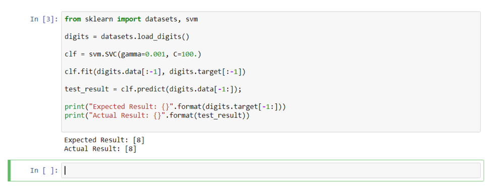
clf.fit(digits.data[:-1], digits.target[:-1])
Once trained, the classifier can be used for classification of digit data. Using the last digit in the dataset, let's invoke the classifier to predict (classify) the digit using the predict method.
Step 1.6 Add the following line of code to the notebook cell:
?test_result = clf.predict(digits.data[-1:]);
Step 1.7 To compare the test_result to the expected result, add the following code to the notebook cell:
?print("Expected Result: {}".format(digits.target[-1:]))
print("Actual Result: {}".format(test_result)
Step 1.8 Finally, run the cell by clicking the "Run" button to see the results.

You should see the expected result and the actual result line up. When this occurs, it indicates that the support vector classifier worked correctly!
Step 2. Testing with Custom Data
In addition to using digits data from the dataset, we can create our own digit data.
Step 2.1 Make a copy of the current "?Predict a Number with Custom Data" notebook using the "File" menu's "Make a Copy" option. Rename the notebook to "Predict a Number with Custom Data".
Step 2.2 Delete all the code that appears after this line of code:
?clf = svm.SVC(gamma=0.001, C=100.)
The notebook cell should look like this:

Step 2.3 Now let's train the support vector classifier with all the digits data. After the assignment of a new instance of a support vector classifier to the clf variable, add the following code:
clf.fit(digits.data, digits.target)
sample_number = [ [ 0., 0., 0., 0., 16., 0., 0., 0. ], [ 0., 0., 0., 0., 16., 0., 0., 0. ], [ 0., 0., 0., 0., 16., 0., 0., 0. ], [ 0., 0., 0., 0., 16., 0., 0., 0. ], [ 0., 0., 0., 0., 16., 0., 0., 0. ], [ 0., 0., 0., 0., 16., 0., 0., 0. ], [ 0., 0., 0., 0., 16., 0., 0., 0. ], [ 0., 0., 0., 0., 16., 0., 0., 0. ], ]
result = clf.predict([[item for sublist in sample_number for item in sublist]])
print(result)
A sample number is a manually-entered number that is not from the training dataset. The range of numbers for each point is 0 to 16. In this example, the digit represented is the number 1. The Python list comprehension passed to the predict method changes the list of lists into a list with a single list.
Step 2.4 Run the notebook cell and observe the results. The number 1 should be the result. So, with new custom data, it predicts (classifies) the correct result.
Step 2.5 Swap out the custom data with additional custom data options:
# number 8
sample_number_8 = [
  [ 0.,  0.,  10.,  14.,   8.,   1.,  0.,  0. ],
  [ 0.,  2.,  16.,  14.,   6.,   1.,  0.,  0. ],
  [ 0.,  0.,  15.,  15.,   8.,  15.,  0.,  0. ],
  [ 0.,  0.,   5.,  16.,  16.,  10.,  0.,  0. ],
  [ 0.,  0.,  12.,  15.,  15.,  12.,  0.,  0. ],
  [ 0.,  4.,  16.,   6.,   4.,  16.,  6.,  0. ],
  [ 0.,  8.,  16.,  10.,   8.,  16.,  8.,  0. ],
  [ 0.,  1.,   8.,  12.,  14.,  12.,  1.,  0. ],
]
# number 1 sample_number_1 = [ [ 0., 0., 0., 0., 16., 0., 0., 0. ], [ 0., 0., 0., 0., 16., 0., 0., 0. ], [ 0., 0., 0., 0., 16., 0., 0., 0. ], [ 0., 0., 0., 0., 16., 0., 0., 0. ], [ 0., 0., 0., 0., 16., 0., 0., 0. ], [ 0., 0., 0., 0., 16., 0., 0., 0. ], [ 0., 0., 0., 0., 16., 0., 0., 0. ], [ 0., 0., 0., 0., 16., 0., 0., 0. ], ]
# number 4
sample_number_4 = [ [0., 0., 0., 0., 16., 0., 0., 0.,], [0., 0., 0., 16., 16., 0., 0., 0.,], [0., 0., 16., 0., 16., 0., 0., 0.,], [0., 0., 16., 0., 16., 0., 0., 0.,], [0., 16., 16., 16., 16., 0., 0., 0.,], [0., 0., 0., 0., 16., 0., 0., 0.,], [0., 0., 0., 0., 16., 0., 0., 0.,], [0., 0., 0., 0., 16., 0., 0., 0.,], ]
Try each number and confirm the results. Did the classifier work as expected?
Step 3. Predict a Number and Display It
In addition to predicting a digit from its image data, the image itself can be rendered with Matplotlib. Displaying the digit image is helpful for visually exploring the effectiveness of the classifier.
Step 3.1 Make a copy of the current "Predict a Number" notebook using the "File" menu's "Make a Copy" option. Rename the notebook to "Predict a Number and Display It".
Step 3.2 Beneath the code to import the datasets and svm, add the following import statement for matplotlib:
from sklearn import datasets, svm
import matplotlib.pyplot as plt
The module matplotlib was installed via the matplotlib package in the first tutorial. Matplotlib is a very popular visualization library. It has an expansive API that can be used to generate publication quality visualizations for research papers and such.
For More Information: https://matplotlib.org/
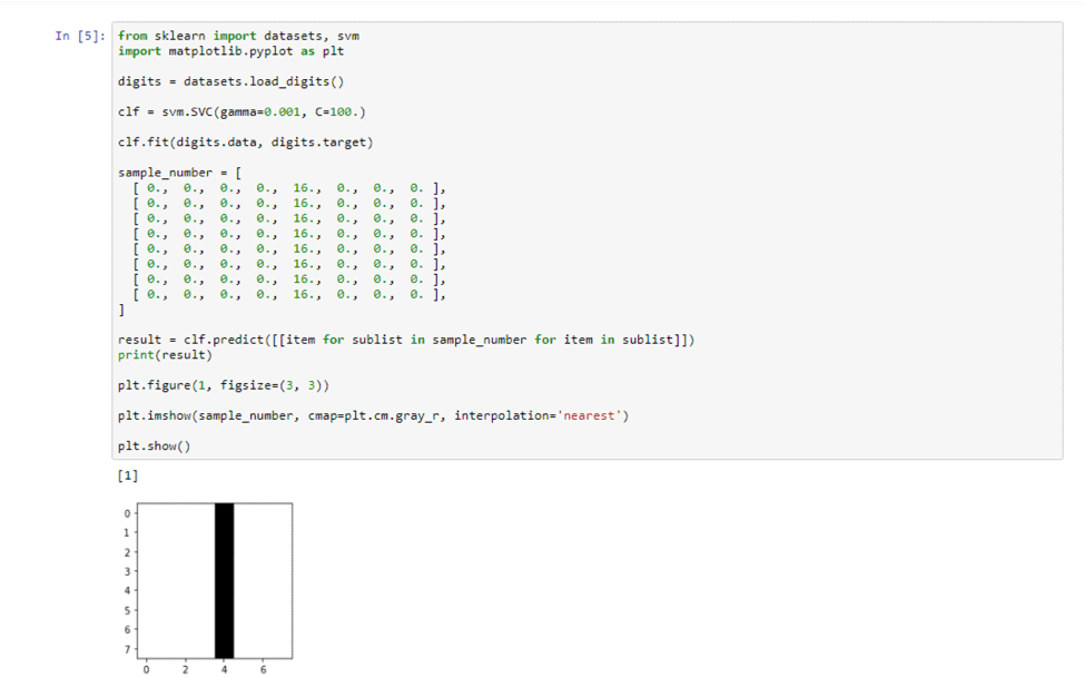
Step 3.3 Add the following code after the call to the predict method to display the sample_number:
plt.figure(1, figsize=(3, 3))

plt.imshow(sample_number, cmap=plt.cm.gray_r, interpolation='nearest')

plt.show()
The visualization of this number should match the output from the support vector classifier.

In this second tutorial, a classifier using a Support Vector Machine was trained and tested. The classifier was able to accept new digit information and properly classify it. Finally, using Matplotlib, the digit data was visualized to aid in the test verification process.
In the next installment of this series, the code will be expanded to load data with Pandas and save/load the trained model. We will then explore how to determine the best hyperparameters for the support vector classifier.

